

The machine learning commands “Train”, “Predict” and “Cluster” explained based on a practical example
Part 2 – „Cluster“ in „ACL™ Robotics“
This is the second part of a short series of blog posts where we present you two machine learning procedures with the analytic Software ACL Robotics. The “ACL™ Robotics” software solution, which has been established on the market for many years, supports the manual and automated analysis of large amounts of data. In addition to a multitude of interfaces to SAP (via “SAP Connector”), Salesforce, Google Hive, Amazon Redshift, Outlook, PDF imports or any ODBC data source, a script language helps to automate analysis steps. The software developer Galvanize allocates this to the field of RPA (Robotic Process Automation). Individual analytic steps are performed by several analytic commands, such as sorting, summarizing, joining and relating, to name only a few. With the Version 14 these analytic commands have been extended by three machine learning commands named as “Train”, “Predict” and “Cluster”. In these two blogposts we will introduce these three commands to you by taking examples from out of the everyday business. For all ACL users, we also offer the opportunity to download ACL projects, allowing you to try out each command, step by step.
This blog post is, due to its length, divided into two parts:
- Part 1 deals with the “Train” and “Predict” commands
- Part 2 deals with the “Cluster” command, which is based on the k-means algorithm
The example for Part 1 was taken from the field of sales: Customers order goods of various different values. Of course, as part of the day-to-day business, this may involve returns. Customers return goods for various reasons and usually receive a refund. In the second part, we are taking up the challenge of dividing customers into groups with similar behaviour. As our example is a B2B example, our customers are likewise companies. As payment term we have agreed on 30 days net, the agreement is stored in the customer master data. Let us take, for example, the following question:
If you grant your customers a payment term of 30 days, are there groups of companies which behave similar towards the deadline?
We will answer this question by using the “Cluster” command in ACL. In Figure 7 you can see a notional dataset of one year plotted. Each point in the graph represents a customer. The annual turnover is plotted on the y-axis. The average payment delay in days is plotted on the x-axis, these values are always rounded. The average always emerges from several payment delays in the reviewed year. An average payment delay of greater than zero means that the invoices of the company observed are, on average, settled prior to the expiry of the 30-day payment period. A value of less than zero means that the respective invoices of the company observed are, on average, paid after the expiry of the 30-day payment period. Companies on the vertical blue line paid, on average, on time, on the last possible day.

Figure 7: Average payment delay in days and annual turnover of 1,449 customers
We are, with the aid of ACL and the “Cluster” command, grouping below the data from Figure 7, in order to answer the question posed at the outset. The “Cluster” function is based on the k-Means algorithm.
Workshop:
- Downloading data: Open ACL and the project “cluster_customers.acl” (download it here for free). This contains the following two tables: “turnover_and_delay” and “turnover_and_delay_with_GAP”. The clustering is carried out below based on the first table. The second table does not, for now, come into the picture.
- Clustering data: Click on “turnover_and_delay” in the side bar. You will now see the associated table in the Basic View. Select “Machine Learning” -> “Cluster”. Next, change the parameters and settings, and then initiate the clustering operation by pressing “OK” (cf. Figure 8).
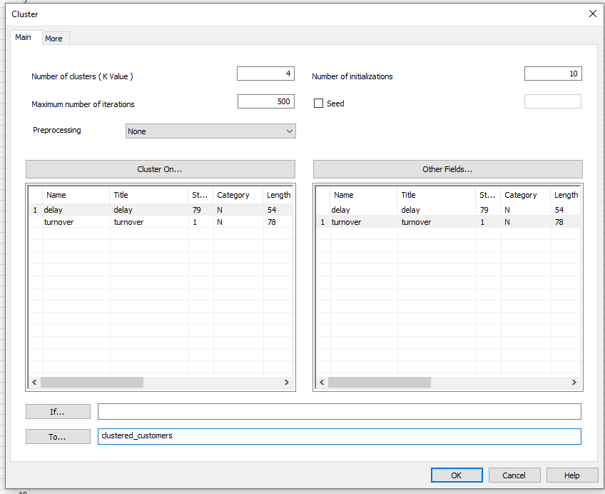
Figure 8: Input mask for clustering with altered parameters
- "Number of clusters (K value)”: This value determines into how many clusters the dataset being inspected is divided. ACL recommends trying out various values. In addition, it is advised to make a first attempt using 8 - 10 clusters. With the aid of Figure 7, we have, in this example, chosen to do 4 clusters.
- “Number of initializations”: K-Means depends upon the starting points selected. For this reason, the algorithm is automatically repeated several times over, using various different starting points, in the ACL software. The best run, i.e. the best clustering, is subsequently selected. “Number of initializations” lets you determine how often the algorithm is supposed to be executed using various different starting points..
- “Maximum number of iterations”: How many iterations should the clustering algorithm carry out per initialization, as a maximum. The higher this value is set, the more suitable are the clusterings resulting from each run.
- “Seed”: K-Means depends upon the randomly selected starting points. “Seed” influences the random number generator. Should you again and again repeat the clustering using the same value for “Seed” and the identical parameters, you will get the same result every time. Should you only change “Seed”, and repeat the clustering, you will get somewhat different clusters each time. This is based on the choice of randomly selected starting values that depend upon “Seed”.
- “Pre-processing”: Here you can edit your fields prior to clustering. This makes sense if your key fields show extreme differences in the value ranges.
- “Cluster on…”: Here you can choose the fields based on which the clusters should be formed. In our case, the average payment delay.
- “Other Fields…”: Here you can specify fields which should be displayed in the results table alongside the aforementioned fields.
- “If…” and “More”: Here you can optionally exclude entries from the dataset.
- “To…”: Here you can specify the name of the results table.
Once the calculation has been completed, you will see the “clustered_customers” table in your side bar. The first k lines in this table always contain the mid-points of the clusters found. The field “Cluster” specifies the associated cluster for each record. The field “Distance” contains the distance to the associated mid-point of the cluster. In Figure 9, the clustering from within the ACL software is visualised by means of colour.
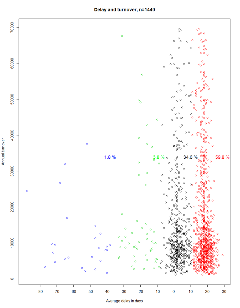
Figure 9: Average payment delay in days and annual turnover of 1,449 customers, clustered into four groups
The clustering generates the following groups:
| Cluster colour | Average payment delay MIN | Average payment delay MAX |
|---|---|---|
| Blue | -88 | -38 |
| Green | -33 | -9 |
| Black | -8 | 10 |
| Red | 11 | 29 |
The blue cluster contains 1.8% of the companies which have paid late in the year observed, on average between 88 and 38 days. For the green cluster (3.8%), the interpretation is made analogously, using the values from the above table. The black cluster contains customers (34.6%) who, on average, paid their invoices on time or not. The red cluster (59.8%) contains exclusively companies which paid on average on time. When looking at Figure 9, it is noticeable that k-Means divides the data into groups relatively well. The clustering nevertheless has a decisive weak point. It would be desirable for every group to be located either fully left or fully right of zero. Interpreting the result is easier if the clusters only contain companies that paid either on average on time or on average not on time. The black cluster is, however, located on both the left and the right side of the zero. For this reason, we use a trick and repeat the above procedure. We generate an artificial gap around zero (cf. Figure 10). All points which are located in the area between -8 inclusive and 0 exclusive, in relation to the x-axis, are moved to exactly x=-8. Points which are located between 0 inclusive and 8 inclusive are moved to exactly x=8.
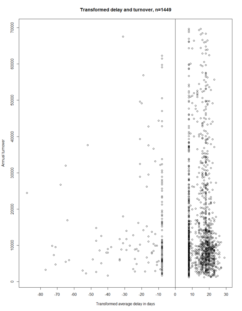
Figure 10: Transformed average payment delay in days and annual turnover of 1,449 customers
We then repeat the clustering in ACL. The resulting grouping can be seen from Figure 11.
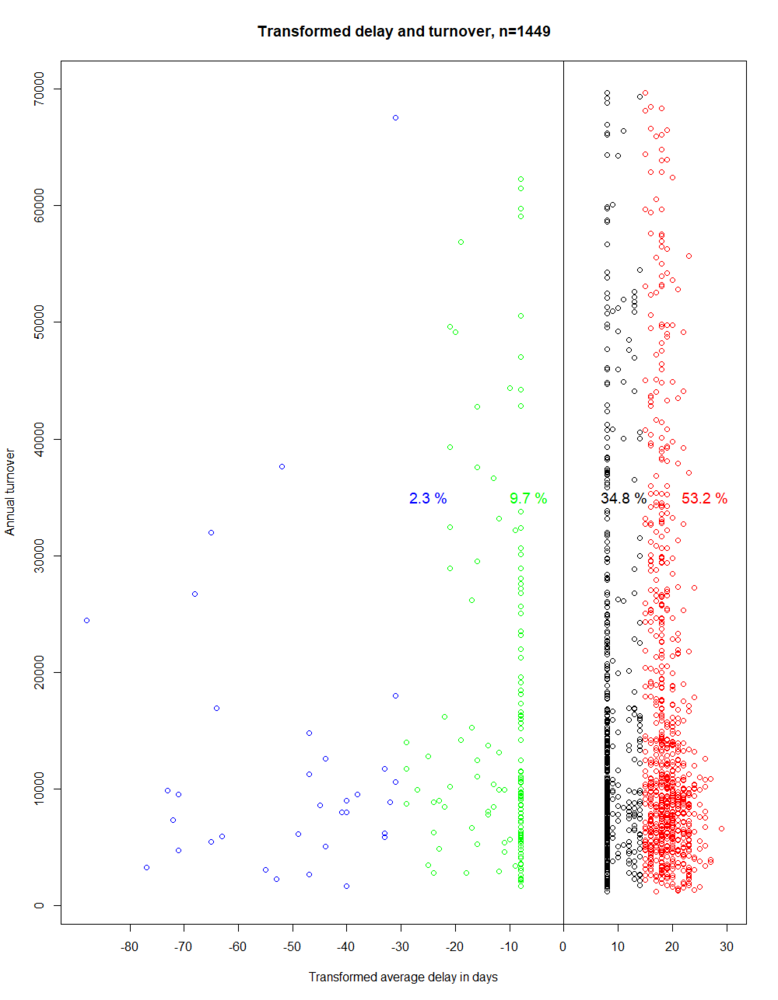
Figure 11: Transformed average payment delay in days and annual turnover of 1,449 customers, clustered into four groups
Using this trick, every cluster is, as desired, located either fully left or fully right of zero. The procedure also works with constants other than -8 and 8. The grouping has been determined by ACL to be as follows:
| Cluster colour | Average payment delay MIN | Average payment delay MAX |
|---|---|---|
| Blue | -88 | -31 |
| Green | -29 | -1 |
| Black | 0 | 14 |
| Red | 15 | 29 |
The grouping can be interpreted as follows: All 1,449 data points can be divided into four sub-sets. On the one hand, 88% of customers, them at the right side of zero, paid on average on time. Whereas, on the other hand, 12% are located to the left of zero - these companies did not, on average, pay on time. On the right-hand side of the zero, the customers were divided into two further groups: Into the black cluster, which contains customers which, on average, paid between 14 days prior to the deadline and the last possible date. The red cluster contains companies which, on average, already paid 29 to 15 days prior to the deadline. The interpretation is made analogously for the green and blue groupings, only paying attention to the changed algebraic sign.
The procedure presented involving the “Cluster” command from ACL belongs to the Unsupervised Learning. In comparison to the example with the estimated return value from Part 1, no value is estimated, but the data is grouped. Thus, no “feature variable” exists.
In this second part of our blog post introducing Machine Learning, we have shown you how you can group your data. The necessary steps you need to perform can be summarised as follows:
- Create a table with the desired “key variables", based on which k-Means is supposed to cluster.
- Carry out the “Cluster” function with suitable parameters
By selecting the “key variables”, as well as said parameters, you can significantly influence the clustering.
We hope you enjoyed reading this blogpost regarding Machine Learning and would be happy, if it can support you, when considering on how to use Machine Learning in your everyday business. Have fun trying out these methods and please do not hesitate to contact us at any time, if you have any questions.