

connect on xing
Turnover analysis
In this article, I would like to show you some possible approaches in order to analyze turnover figures of vendors and customers and which questions are relevant. The analyses are shown by means of the analysis software ACL™ Analytics.
Structure of table LFC1
The vendors’ turnover figures are displayed in table LFC1 per vendor number (field LIFNR), company code (field BUKRS) and fiscal year (field GJAHR). The balance carried forward at the beginning of the fiscal year is stored in the field UMSAV; this corresponds to the open amount which was not cleared in the previous year. The subsequent fields are listed per period, this means 16 times. XX is the placeholder for the current period. One posting period corresponds to one month, periods 13 – 16 are special periods where year-end closing postings are done:
- LFC1_UMXXS: Sum of the debit postings in the period
- LFC1_UMXXH: Sum of the credit postings in the period
- LFC1_UMXXU: Turnover in the period. The field includes the sum of all sales-related postings in this posting period. It depends on the posting key if a posting is sales-related. For instance, a vendor invoice is sales-related whereas a payment is non-sales-related; this means that it is not relevant for the turnover amount if a vendor invoice has been already cleared.
The following example displays transaction figures of vendor 111 in the transaction SE16. For visualization reasons, the view was separated to two screenshots:

Figure 1: Structure of table LFC1: First part
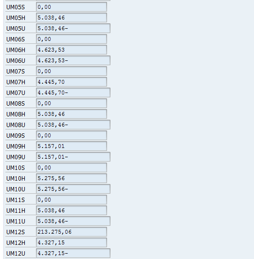
Figure 2: Structure of table LFC1: Second part
In this example, the balance carried forward had a credit amount of 158,385.48 Euro at the beginning of fiscal year 2004. A negative amount represents credit postings whereas a positive amount represents a debit posting. The balance carried forward was calculated by making the balance of all debit postings and credit postings in the previous year.
Furthermore the sum of the credit and debit postings as well as the sum of the turnover is listed for each period. You see in this example that turnovers are only displayed with a negative amount. As already mentioned, credit postings are totaled as negative amount. Since the credit sum is always corresponding to the turnover sum, the credit postings were always sales-related. In period 12, the sum of the debit postings had an amount of 213,275.06 Euro. Since this amount did not influence the turnover in period 12, the debit postings were not sales-related.
Analysis of vendors’ turnover figures in ACL™ Analytics
In this chapter, the turnover trend will be looked at. First and foremost the following aspects will be regarded:
- Which vendors had the highest turnovers?
- Which vendors had the highest deviations?
The analyses are shown by means of ACL™ Analytics. We can use table LFC1 as basis for the turnover figures. Since we are interested in the total turnover per year, we create a calculated field c_Turnover which totals the turnovers of all periods. Since the turnovers are shown with a negative amount, the sum is multiplied by (-1).

Figure 3: Calculation of the turnover per year
In the first analysis, the vendors with the highest turnover in company code 1000 from the years 2005 – 2008 should be identified. First, the turnover per vendor must be totaled by vendor, filtered to company code 1000. In our example, customer 1075 has the highest turnover: rder value.

Figure 4: Vendors with the highest turnover
A further interesting aspect is to analyze the turnover trend per vendor and identify huge deviations. In the following example, the turnover of two fiscal years will be compared. In table LFC1, the fiscal years are listed one below the other; therefore the comparability is difficult. By means of the CROSSTAB command, it is possible to list the turnover figures side by side. For to keep the example easy to read, only two fiscal years (2005 – 2006) will be compared. Field LFC1_LIFNR is selected as row whereas field LFC1_GJAHR is selected as column.
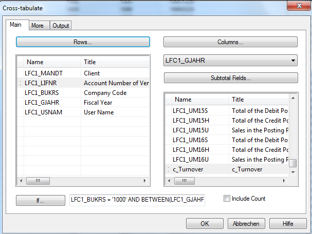
Figure 5: CROSSTAB command on LFC1
In the result table, a column is created for each fiscal year to make turnover per fiscal year visible.
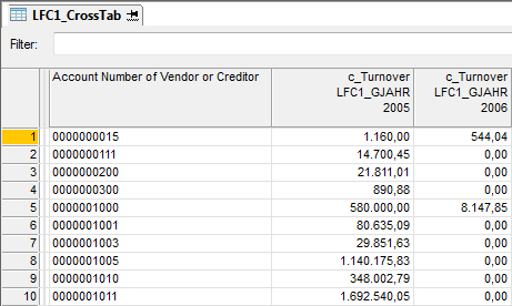
Figure 6: Result table after the CROSSTAB command
To compare the turnover figures in the years 2005 and 2006, we create a calculated field c_Dif_Turnover which subtracts the turnover in year 2005 from the turnover in year 2006. To identify the hugest turnover increases, the result table is sorted descending by the difference. We get the following table as result.

Figure 7: Turnover differences between the years 2005 and 2006
Analysis of customers’ turnover figures in ACL™ Analytics
The customers’ turnover figures are stored in table KNC1. In contrary to vendors, the turnovers are displayed with a positive amount here. Therefore the annual turnover per customer is calculated the following way:

Figure 8: Turnover analysis in KNC1
The subsequent analyses are analog to table LFC1; therefore a further description is not necessary.
Conclusion
This article has shown with two examples which analysis possibilities exist in table LFC1/KNC1. In the first example, the total turnover of the vendor/customer was calculated; in the second example, the absolute increase of the turnover within a year was calculated. Indeed, we can get more information from these tables and make further analyses. A complete vendor ranking or customer ranking bases mostly on the turnovers in a longer period and analyses their trends.
If you have any questions on this topic or want to place a comment, feel free to contact me on info@dab-gmbh.de.